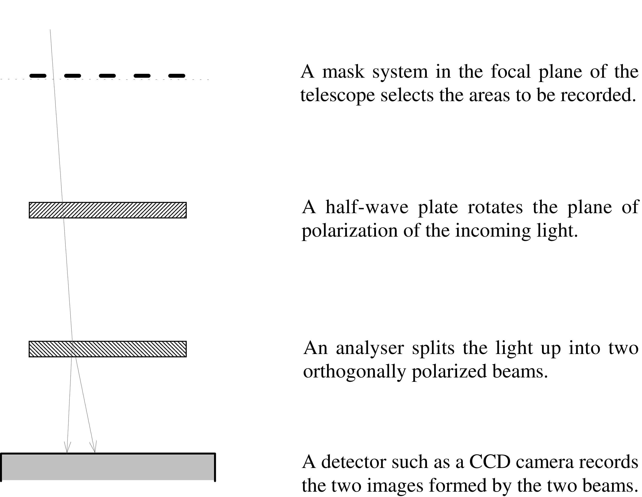
Figure 1: The main optical components in a typical dual-beam imaging polarimeter.
This section gives a brief introduction to the general principles of dual-beam polarimetry. It explains words and concepts used later, and defines the data model used by POLPACK. A well established example of a dual-beam polarimeter is described by Scarrott et al. (Mon. Not. R. astr. Soc. (1983) 204, 1163 - 1177).
Single waveband polarimetry is described here but the principles can be extended to imaging spectropolarimetry (see section 4).
A dual-beam polarimeter suitable for measuring linear polarization usually contains the following optical components:
The light collected by the telescope passes through these components in the order listed (see Figure 1). Each component is described more fully below.
The heart of the polarimeter is the analyser, which splits incoming partially plane polarized light up into two beams; one (called the ordinary, or ray) contains the component of the incoming light which is polarized parallel to the axis of the analyser, and the other (called the extraordinary, or ray) contains the component of the incoming light which is polarized orthogonally to the axis of the analyser. These two beams are recorded simultaneously on a suitable detector such as a CCD. The advantage of this system over a single-beam instrument (in which only one state of polarization is recorded on a given exposure), is that variations in sky background between exposures affect both states of polarization equally, and so can be eliminated.
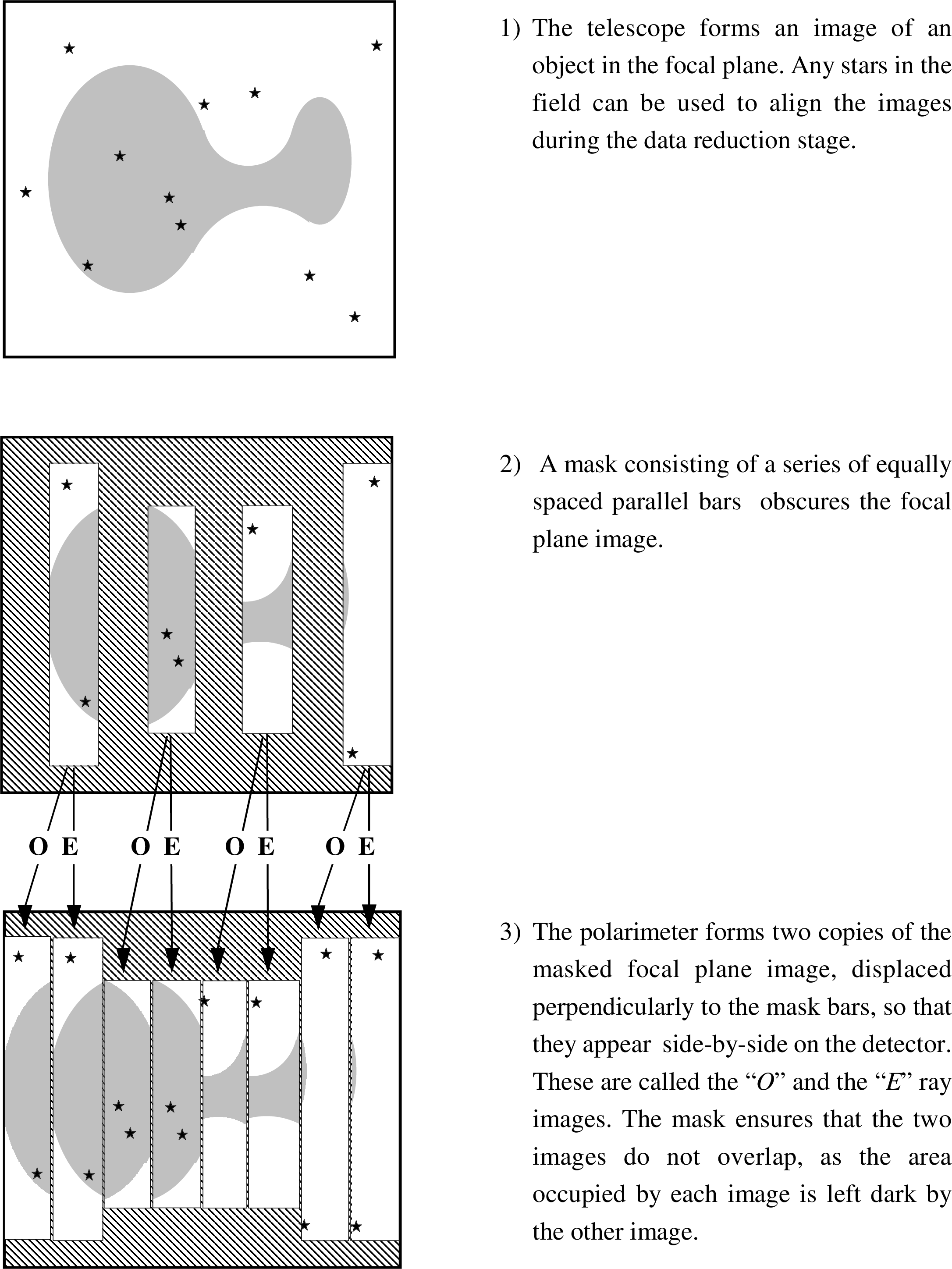
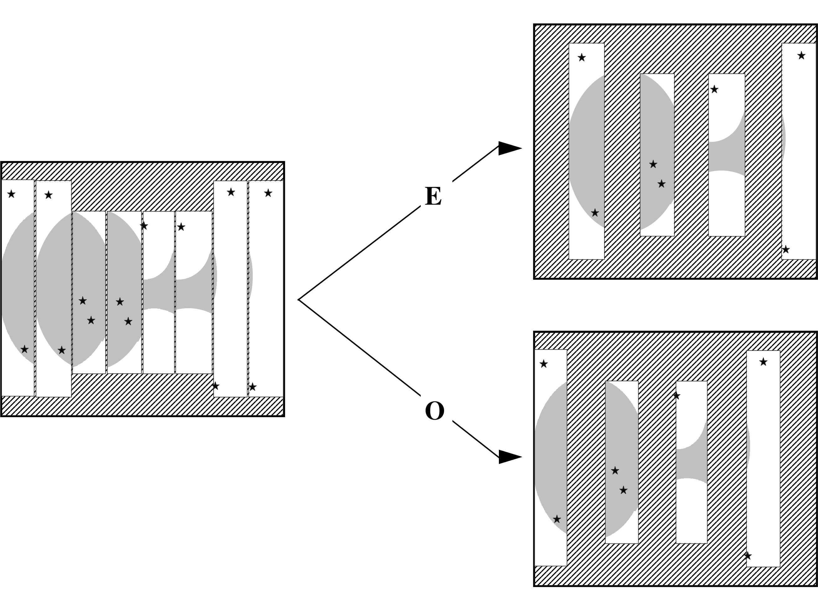
In an imaging polarimeter, the two beams form two images on the detector, displaced by some distance determined by the design of the instrument; both images representing the same area of the sky. A masking system is used to prevent any overlap between the two images. In some instruments this takes the form of a series of parallel, equally spaced bars in the focal plane of the telescope (see Figure 2). In this case, the instrument is designed so that the displacement between the two images formed by the and rays is perpendicular to the bars, and equal in size to the width of a bar. Thus, the two images form two inter-leaving sets of bars. There are several other systems (such as a mask containing only a single aperture), but the principle is the same.
If the incoming light is only partially polarized, then at least two exposures are required to estimate both the degree and the orientation of the polarization, each exposure recording the intensity in two orthogonal states of polarization as described above. The analyser axis is rotated in steps of 45° between these exposures. In practice, physically rotating the analyser would result in the displacement between the and the ray images also rotating. This would cause the images to overlap on the detector and would make the data reduction process much harder (if not impossible). For this reason, the analyser is usually left in a fixed position, and the plane of polarization of the incoming light is rotated instead. This is achieved by placing a half-wave plate in front of the analyser, and rotating it in steps of 22.5° , resulting in a rotation of the plane of polarization of 45° . Using this scheme the positions of the and ray images on the detector are unchanged.
The orientation of the plane of polarization of the incoming light is measured relative to a fixed “reference” direction. The analyser axis and the 0° position of the half-wave plate are usually parallel to this direction.
At least two exposures are required to estimate the degree and orientation of the polarization, taken with half-wave plate positions of 0° and 22.5° (see appendix B). For ease of reference, these exposures are referred to here as and . The and ray images in measure the intensities parallel and perpendicular to the reference direction. has an effective analyser angle of 45° (twice the half-wave plate angle) and so measures the intensities at angles of 45° and 135° to the reference direction
Usually, a further two exposures are taken at half-wave plate positions of 45° and 67.5° (referred to here as exposures and ). These provide some redundancy in the data and enable internal consistency checks to be made during the data reduction stage.
These exposures are denoted by the letter to indicate that they are target exposures. In addition to these target exposures, some flat-field exposures are also required. These are used to correct for any spatial variation in the sensitivity of the system, and consist of exposures of a photometrically flat surface. Ideally, the flat-field source should be unpolarized. However, if the additional target exposures and are taken, then a spatially constant polarization across the flat-field source can be corrected for during data reduction. Since the polarization of the flat-field surface is rarely known to be zero, these additional target exposures should always be taken.
It is important that the flat-field has a good signal-to-noise ratio. For this reason, it is common practice to take one or more flat-field exposures at each half-wave plate position, and stack them together into a single master flat-field (although it is not strictly necessary to use different half-wave plate positions). Further discussion of the flat-fielding procedure is given in section 2.3.1.
Several steps are involved in the production of a polarization map from the raw exposures recorded by the detector. An over-view of these steps is given here. Details of how they may be implemented in practice using POLPACK are given in later sections of this document.
These convert the raw data numbers measured by the detector into values which are proportional to the combined sky and object intensity transmitted by the analyser (plus noise of course). The details of these corrections will depend on the nature of the detector. For a CCD camera, they will usually involve at least flat-fielding, and de-biassing.
Flat-fielding is worthy of some extra discussion, since it can be complicated by the presence of the polarimeter in the light path. The purpose of flat-fielding is to ensure that there are no spatial variations in the sensitivity of the detector. This is normally achieved by taking images of a photometrically flat surface such as the inside of the observatory dome, or the twilight sky3. Since the brightness of this surface is constant, any variations in the recorded image (the “flat-field” image) must be due to variations in the sensitivity of the detector. These variations can then be removed from the target observation by dividing every pixel value in the target image by the corresponding pixel value in the flat-field image.
Introducing a polarimeter into the light path can complicate this if the flat-field is taken in polarized light (such as is produced by reflective surfaces in the dome, or by light scattering in the atmosphere). In this case the intensity of the light reaching the detector will not be constant across the field, but will depend on the polarization.
If the polarization of the flat-field is non-zero and spatially constant, then the and ray flat-field images will have different mean values (visible as sharply defined dark and light areas in the flat field). If such a flat-field is used to correct the target exposures, then the different mean values in the flat-field will result in an apparent difference in sensitivity between the two channels of the polarimeter (known as the “F-factor”). Such a difference in sensitivity can be corrected for when calculating the polarization if the additional target exposures and (see section 2.2) are available.
Note, the same flat-field should be used to flat-field all target exposures, irrespective of half-wave plate position.
A mathematical description of the flat-fielding and F-factor corrections is given in appendix C.
Each exposure contains two images of the same area of the sky: the and the ray images. Once any detector corrections have been applied, these images need to be identified and extracted into two separate arrays for further processing.
The arrays holding the extracted and ray images now need to be aligned so that the same pixel in each array corresponds to the same position on the sky. This can usually be achieved by aligning stars within the arrays.
The intensity of the background night sky now needs to be estimated and subtracted from each of the aligned arrays. The sky may be polarized, and so this needs to be performed independently within each of the aligned arrays.
The Stokes parameters , and are all measures of intensity, and together provide a useful description of the polarization of the object being studied. Since , and all have the same units, this description is generally easier to use than the more obvious description given by the degree of polarization and the orientation of the plane of polarization. The mathematical connection between the Stokes parameters and the sky-subtracted intensities is described in appendix B. The output from this stage of the reduction process is a Stokes vector (i.e. a set of , and values) for each measured pixel on the sky.
One consequence of the fact that the Stokes parameters , and are all measures of intensity, is that they can be binned spatially. This not only produces less confusing polarization maps (due to the reduced number of measurements), but also improves the signal-to-noise ratio.
The use of Stokes parameters to describe polarization has mathematical advantages, but is not easy to represent in a graphical manner. For human interpretation therefore, polarization is usually described by the degree of polarization, , (i.e. the ratio of polarized to total intensity), and the orientation of the plane of polarization, . Note, is the angle between the plane of polarization and the reference direction of the polarimeter. To convert this to a position angle on the sky, the position angle of the reference direction must be known. The simplest way to derive these parameters from the Stokes parameters is as follows:
where is the polarized intensity. However, the estimation of is complicated by the non-symmetric noise statistics produced by squaring and adding and . For low polarizations, the squaring of the noise will tend to shift the mean of the distribution of to higher values, thus resulting in an over-estimation of . The use of the following expression for reduces the effect of this statistical bias:
where is the variance on or (which are assumed equal). A description of the statistical behaviour of polarization parameters is given by Serkowski (Advances in Astronomy and Astrophysics, ed. Z. Kopal, Academic Press, New York, London (1962), 1, 304).
The final polarization parameters are usually presented graphically in the form of a polarization map (see the first page of this document for an example). Each measurement is represented as a vector parallel to the plane of polarization. The length of the vector is proportional to the degree of polarization, which varies from 0% to 100%. The Stokes vectors can be binned to reduce the number of vectors in the map to a manageable number. The map is often overlayed on a total intensity image or contour map of the object to emphasize any correlation between the visual appearance of the object and the morphology of the polarization map.
3In the near infra-red flat-fields are normally taken on the night sky which at these wavelengths is bright enough to give a good signal to noise ratio.